Secondary Comparison Pressure Standards
A secondary comparison pressure standard is any device that measures pressure which does not meet the criteria of a primary pressure standard. Secondary pressure standards therefore comprise both mechanical and electronic instruments with varying rates of measurement accuracy.
In general, secondary pressure standards have the following advantages in comparison to primary pressure standards:
1. Faster and easier to use
2. Usually no measurement corrections
3. Non-incremental measurements
4. Generally less expensive
In general, secondary pressure standards have the following disadvantages in comparison to primary pressure standards:
1. Must be periodically recalibrated by a primary pressure standard traceable to national standards
2. Pressure measurements cannot be reduced to measurements of mass, length or temperature
6.1 Types of Secondary Pressure Standards
6.1.1 Mechanical Pressure Gauges
The most commonly used secondary pressure standard is the mechanical pressure gauge. This instrument utilizes a hollow tube (Bourdon) that is formed into the shape of a C, a spiral or a helix. When pressure is applied within the tube, the tube tends to straighten out. This movement is transferred to a display pointer either through a gear rack and pinion mechanism or a direct drive.
The measurement accuracy of mechanical pressure gauges varies generally from 3% full scale to 0.10% full scale. The higher accuracy gauges are known as “Test gauges”. The hollow tubes are generally manufactured from nonferrous materials such a beryllium copper, Monel, stainless steel and Nispan “C”. Other mechanical pressure gauges use diaphragms and capsules to expand with the applied pressure.
The bourdon tube can also be constructed from a stable material such as quartz to achieve higher levels of measurement accuracy. Accuracies will vary with the manufacturer, but accuracies as high as 0.015% Full Scale are available.
6.1.2 Electronic Pressure Gauges
The electronic pressure standards comprise a large, divergent group of instruments with widely varying features and accuracy. Each of these instruments incorporates a pressure transducer. The function of which is to convert an input pressure signal to an electronic signal such a resistance, voltage, current etc. The most common transducers incorporate an electronic strain gauge and a wheat stone bridge generally located on a silicon chip. Other transducers incorporate piezo electric, vibrating wire or cylinders and other technologies.
The advantages of these instruments is that they display the pressure on easily read digital displays, are easy to use and are generally small, light in weight and portable. On the negative side, the secondary standards are generally not as accurate as primary standards and the accuracy is seriously affected by temperature variations.
In most cases, the overall accuracy of the instrument is divided into several elements such as:
1. Accuracy, % Full Scale or % Indicated
Reading
2. Precision, Repeatability, Hysteresis
3. Temperature Effect
4. Resolution
It is important when selecting a secondary pressure standard, therefore, to consider first the application task to be performed and then to evaluate the overall accuracy capabilities of each instrument.
6.2 Overall Application Accuracy
Many different elements must be combined to establish the overall application accuracy of an instrument when performing a specific test. These elements include the accuracy measurement, repeatability, hysteresis, linearity, temperature affect, resolution and laboratory uncertainty. Each of these elements is described within the following paragraphs.
6.2.1 Application Task
When evaluating the overall accuracy of an instrument, the first item that must be considered is the application or task for which the pressure standard will be used. Elements that should be considered are the minimum and maximum pressures to be measured and the minimum and maximum ambient temperatures within which the instrument will be used.
For purposes of illustration we have selected an application where the customer wishes to measure pressure over a range of 4″ H2O (20°C) to 200″ H2O with ambient temperature variations from 20° to 110°F (-7° to 43°C).
6.2.2 Accuracy Measurement
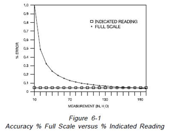
The measurement accuracy of instruments is generally expressed as “Per Cent of Full Scale” or “Percent of Indicated Reading”. As illustrated on Figure 6-1 if the accuracy of a 200 inch of water column capacity instrument is stated as +0.05% full scale, the guaranteed accuracy is +0.1 inch of water column throughout the operating range. If the instrument is used at 10 inches of water, the accuracy of measurement is 1%. If on the other hand the accuracy of the same 200 inch of water column instrument is stated as +0.05% indicated reading, the accuracy at 200 inches of water column would still be +0.1 inch of water but the accuracy at 10 inch of water column would be +0.005 inch of water column.
As an example of this calculation, consider an electronic pressure gauge (A) with a specified range from 0 to 280″ H2O, a stated accuracy of 0.1% full scale plus 1 Least Significant Digit. For the application of 4″ H2O to 200″ H2O, the accuracy portion of the overall application accuracy at the 4″ and 25″ H2O test points would be:
Specified error:
280″ H2O (Full Scale) x 0.1% = 0.28″ H2O
Less Significant Digit = 0.1″ H2O
Total = 0.28 + 0.1 = 0.38″ H2O
Application error @ 4″ H2O:
0.38″ H2O / 4 x 100 = 9.5 %
Application error @ 25″ H2O:
0.38″ H2O /25 x 100 = 1.52%
As a further example of an electronic pressure gauge, consider an instrument (B) with an operating range of 0 to 5 PSIG, a stated accuracy of +0.03% full scale plus 0.07% of the indicated reading plus 1 Least Significant Digit. The accuracy portion at the 4″ and 25″ H2O test points would be:
Specified error:
5 PSI x 27.72″ H2O/PSI x 0.03% =0.04158″ H2O
0.07% indicated Reading x 25″ H2O = 0.0175″ H2O
or
0.07% indicated Reading x 25″ H2O = 0.0175″ H2O
Least Significant Digit = 0.001″ H2O
Total @ 4″ H2O = 0.04538″ H2O
Total @ 25″ H2O = 0.06008″ H2O
Application error @ 4″ H2O:
0.04538″ H2O / 4 x 100 = 1.1345%
Application error @ 25″ H2O:
0.06008″ H2O /25 x 100= 0.24032%
Consider as a further example a deadweight tester with a specified range of 250″ H2O and a stated accuracy of 0.015% of the indicated reading.
Since the accuracy is stated as percent of indicated reading, the application error at both the 4″ and 25″ H2O test points would be 0.015%.
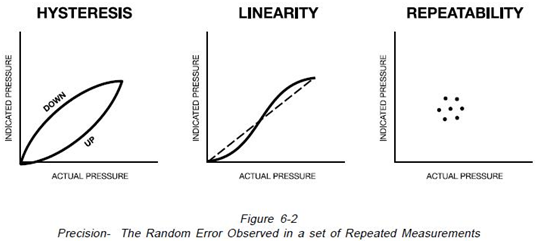
6.2.3 Hysteresis, Linearity, Repeatability
As illustrated on Figure 6-2, hysteresis is defined as the maximum difference for the same measured quantity between the upscale and the down scale readings during a full range traverse in each direction. Linearity is defined as the maximum deviation of the instrument characteristics from a corresponding point on a specified straight line. If the straight line does not pass through zero, the difference between the location of the line and zero is defined as “Zero Offset”. Repeatability is defined as the closeness of agreement among a number of consecutive measurements of the output of an instrument for the same value of the input under the same operating conditions, approaching the measurement from the same direction, and for full range traverses. This term is identical to the statistical “Precision” of a measurement. In general, the combined error from hysteresis, linearity and repeatability is stated as a single error percentage in instrument specifications.
Continuing the example, the hysteresis, linearity and repeatability are included within the accuracy specification of most of the electronic digital gauges, therefore the incremental contribution of both the example (A) and (B) gauges to the overall accuracy of these instruments is zero.
For the deadweight tester, the repeatability or precision is usually specified as a separate portion of the accuracy statement. For the example the repeatability of the deadweight tester is estimated at 0.005% of the indicated reading.
6.2.4 Temperature Effect
The “Temperature Coefficient” is a measure of the change of a parameter as a result of a change in ambient temperature. It is generally expressed as a percentage change in the parameter per degree of change (Percent/ °C or Percent/°F).
The electronic digital gauge (A) example is not temperature compensated. The temperature coefficient is specified as 0.01% full scale per °F. The calibration temperature is 68°F. The maximum application temperature difference is:
68°F – 20°F = 48°F
Temperature error = 48°F x 0.01% = 0.48% full scale
0.48 % full scale x 280″ H2O (Full scale) = 1.344″ H2O
Application temperature error @ 4″ H2O =
1.344″ H2O/ 4″ H2O(Low Application Pressure) x 100 = 33.6 %
Application temperature error @ 25″ H2O =
1.344″ H2O/25″ H2O x 100 = 5.376 %
Electronic pressure gauge (B) is temperature compensated over a range of 20° to 130°F (-7 to 54°C). The temperature coefficient portion of the overall efficiency is zero.
The deadweight tester is not temperature compensated but has a very low temperature coefficient. The temperature coefficient is 0.0009278%per °F. The calibration temperature is 73.4°F.
The maximum application temperature differential is:
73.4°F – 20°F = 53.4°F
Temperature error =
53.4°F x 0.0009278% = 0.049%
Application temperature error =
(4″ and 25″ H2O) = 0.049%
6.2.5 Resolution
Resolution is defined as the least incremental value of input or output that can be detected, caused, or otherwise discriminated by the measuring device. This parameter is best illustrated by the following example of a 100 PSI capacity instrument. At 100 PSI, if the instrument has 3 digits, it can display only 99.6 to 100.4 PSI with a potential resolution error of .4%. If the display is 4 digits, the error is reduced to 99.96 to 100.04 PSI or 0.4%. A five digit display reduces the error to 99.996 to 100.004 PSI or 0.004%. However, with the same instrument, if the measurement is measuring
10 PSI the 3 digit measurement is 9.6 to 10.4
PSI or 4%, the 4 digit instrument is 9.96 to 10.04
PSI or 0.4% and the 5 digit measurement is 9.996 to 10.004 PSI or 0.04%.
Resolution error is not additive to other error parameters but the overall error can never be less than the instrument resolution at the lowest point of measurement.
The electronic digital pressure gauge (A) has a 3 1/2 digit display with one decimal maximum (0.1″ H2O). The maximum resolution error is therefore:
4″ H2O:
0.1″ H2O / 4″ H2O x 100 = 2.5%
25″ H2O:
0.1 H2O / 25″ H2O x 100 = 0.4%
Electronic pressure gauge (B) has a 5 digit display with a 3 decimal maximum (0.001″ H2O).
Maximum resolution error is therefore:
4″ H2O:
0.001″ H2O / 4″ H2O x 100 = 0.025%
25″ H2O:
0.001″ H2O /25″ H2O x 100 = 0.004%
The deadweight tester does not have a display, therefore the resolution error component of the overall application accuracy is not applicable.
6.2.6 Stability
Stability is defined as the ability of an instrument to maintain the measurement accuracy over a specified time period. All instruments must be calibrated after some time interval to assure that the accuracy performance has not degraded.
The shorter the stability time period, the more frequently the instrument must be recalibrated.
Recalibration of some instruments can be done by the customer while other types must be returned to the manufacturer.
The stability or frequency of calibration requirement is seldom included within the advertised literature for secondary pressure standards. Users frequently must consult the manufacturer for recommended intervals.
6.2.7 Laboratory Uncertainty
Laboratory uncertainty is defined as the ability or certainty of a laboratory to measure the specific parameters necessary to establish the various elements of the instrument accuracy. Currently this measure is only applied to national standards laboratories such as United States National Institute of Standards and Technology and a few manufacturers of equipment for primary standards laboratories. A world wide program is underway to accredit laboratories with regard to their capability. This measure should become more important in the future.
6.2.8 Overall Accuracy
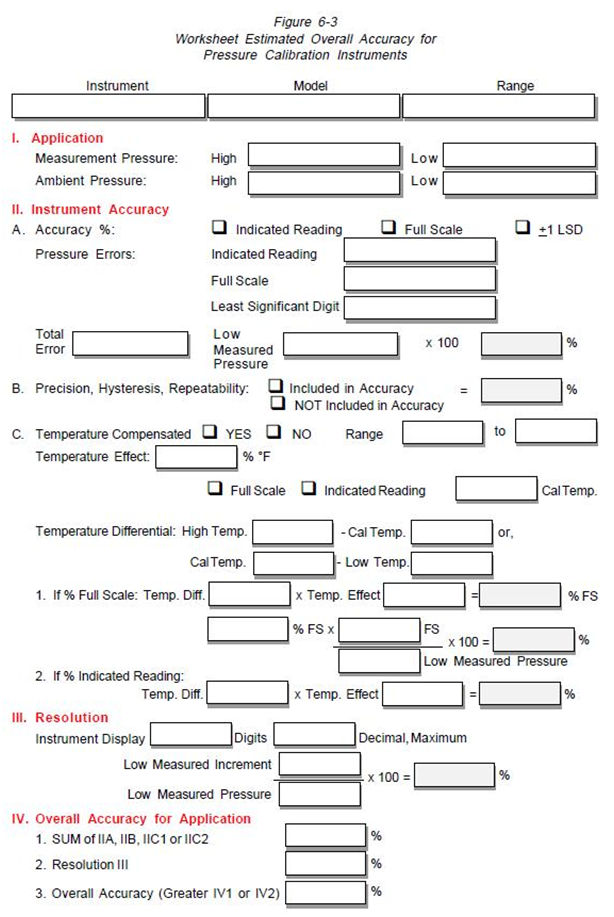
In order for the user to determine the overall accuracy of measurement for each application it is necessary to consider all of the elements contributing to the accuracy of measurement together with the minimum and maximum pressure and ambient temperatures for the planned application.
A Worksheet for Estimated Overall Accuracy is shown on Figure 6-3. This worksheet can be used to evaluate alternate instruments for individual applications.
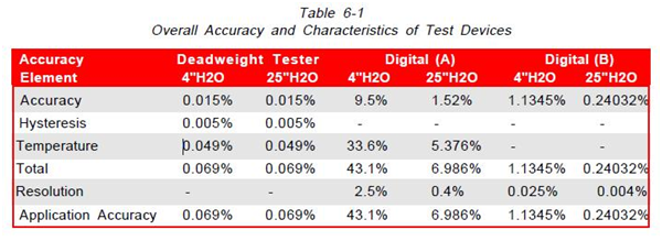
For the three instruments that have been used for the example, the overall accuracy at the 4 and 25 inch H2O test conditions are as follows:
Source: Ametek